Analysis becomes a serious tool for partial differential equations the moment a computation turns into an inequality that survives limits. A priori estimates are not decoration. They are the mechanism that replaces exact formulas when formulas do not exist, and they are the bridge between formal manipulation and existence, uniqueness, stability, and qualitative structure.
A useful way to read much of modern PDE is to track a small number of estimate types and watch how they combine:
Value WiFi 7 RouterTri-Band Gaming RouterTP-Link Tri-Band BE11000 Wi-Fi 7 Gaming Router Archer GE650
TP-Link Tri-Band BE11000 Wi-Fi 7 Gaming Router Archer GE650
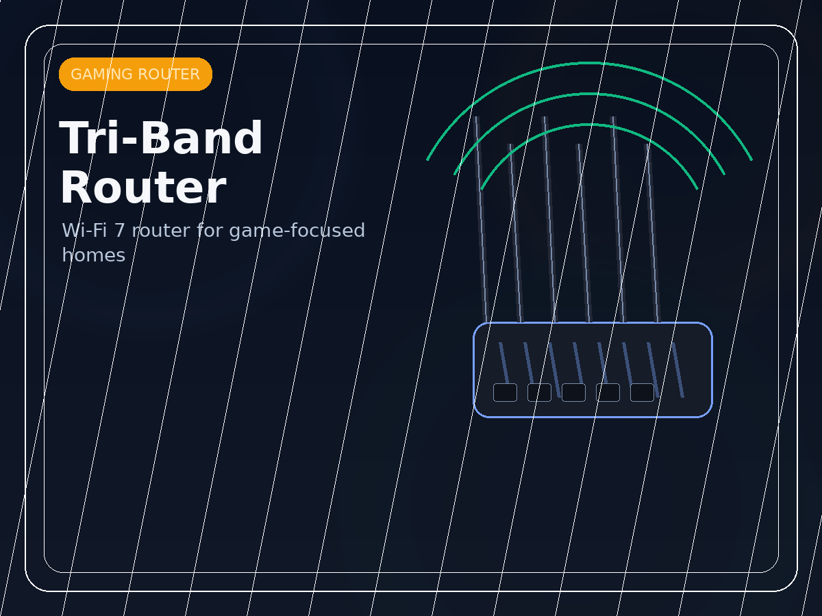
A gaming-router recommendation that fits comparison posts aimed at buyers who want WiFi 7, multi-gig ports, and dedicated gaming features at a lower price than flagship models.
- Tri-band BE11000 WiFi 7
- 320MHz support
- 2 x 5G plus 3 x 2.5G ports
- Dedicated gaming tools
- RGB gaming design
Why it stands out
- More approachable price tier
- Strong gaming-focused networking pitch
- Useful comparison option next to premium routers
Things to know
- Not as extreme as flagship router options
- Software preferences vary by buyer
- Energy estimates that come from multiplying an equation by a strategically chosen test function and integrating by parts.
- Maximum principle estimates that turn sign information into uniform bounds.
- Compactness and interpolation estimates that turn boundedness in one norm into convergence in another.
The worked examples below are chosen because each one exhibits a pattern that repeats in far more technical settings.
Example A: Poisson’s equation and the first energy estimate
Consider a bounded domain $\Omega\subset\mathbb{R}^d$ with sufficiently regular boundary and the Dirichlet problem
The defining estimate comes from the formal identity
Integrating by parts and using the boundary condition yields
Now apply Cauchy–Schwarz:
To turn this into a bound on $\nabla u$, use Poincaré’s inequality for zero boundary data:
Combine these:
So
This estimate already encodes three foundational lessons.
- **The estimate is in the right space.** The Dirichlet problem naturally produces a bound in $H^1_0(\Omega)$ rather than in $C^2$.
- The boundary condition is part of the inequality. Poincaré fails without anchoring, so the estimate is inseparable from the geometry of the boundary condition.
- Existence can be obtained by minimizing an energy. Define the functional
on $H^1_0(\Omega)$. The estimate above is the coercivity that makes minimization work.
In a single computation, you see how PDE becomes functional analysis.
Example B: The heat equation and dissipation
Let $u=u(t,x)$ solve the heat equation on $\Omega$ with zero Dirichlet data:
Multiply by $u$ and integrate over $\Omega$:
The first term is $\frac12\frac{d}{dt}\|u\|_{L^2(\Omega)}^2$. The second term becomes $\|\nabla u\|_{L^2(\Omega)}^2$ by integration by parts. Therefore
Integrate in time from $0$ \to $T$:
This identity carries more information than it first appears \to.
- $\|u(t)\|_{L^2}$ is nonincreasing, so the flow is stable in $L^2$.
- The integral of $\|\nabla u\|_{L^2}^2$ is controlled, so the solution gains spatial regularity on average in time.
- If two solutions start close in $L^2$, the same identity applied to the difference proves uniqueness.
A standard refinement uses Poincaré again:
where $\lambda_1$ is the first Dirichlet eigenvalue. Then
so $\|u(t)\|_{L^2}\le e^{-\lambda_1 t}\|u(0)\|_{L^2}$. No explicit heat kernel is needed to see exponential relaxation on bounded domains.
Example C: A transport term and Grönwall’s inequality
A wide class of PDE has the shape
for a vector field $b$. The transport term is neither dissipative nor smoothing. The estimate that replaces dissipation is a controlled growth inequality.
Assume $b$ is smooth and divergence-free, $\nabla\cdot b=0$, and take $L^2$ inner product with $u$. Using integration by parts,
With a no-flux boundary condition $b\cdot n=0$ and divergence-free $b$, this term vanishes. Then
So
The solution is stable, but not contractive.
If $\nabla\cdot b\neq 0$, the estimate becomes a growth law. A basic bound is
which yields
At this point, Grönwall’s inequality becomes the estimate engine. In more delicate settings, transport estimates are the gateway to well-posedness under minimal regularity assumptions on $b$, and the proof is essentially a careful version of this computation.
Example D: A nonlinear elliptic estimate and the role of monotonicity
Consider the semilinear equation
with zero Dirichlet boundary condition, where $g$ is monotone increasing and satisfies $g(0)=0$. Multiply the equation by $u$ and integrate:
Monotonicity implies $g(u)u\ge 0$, so
So $\|\nabla u\|_{L^2}\le C\|f\|_{L^2}$ again. The nonlinear term does not break the estimate because it has a sign. This is a recurring phenomenon: the right structural assumption is not smoothness of the nonlinearity but coercivity or monotonicity.
A second estimate comes from testing with $g(u)$ itself. Under mild growth assumptions, this can control $\|g(u)\|_{L^2}$ and yield bounds that survive approximation.
Example E: The wave equation and conserved energy
For the wave equation
with Dirichlet boundary condition, multiply by $\partial_t u$ and integrate:
The first term is $\frac12\frac{d}{dt}\|\partial_t u\|_{L^2}^2$. The second term becomes $\frac12\frac{d}{dt}\|\nabla u\|_{L^2}^2$. Thus
The conserved quantity
is the wave energy. Unlike the heat flow, there is no dissipation. That difference is not philosophy, it is an estimate statement.
From this identity you get uniqueness, continuous dependence on initial data, and global existence for the linear equation. In semilinear wave equations, this energy is also the starting point for blow-up criteria and scattering theory, depending on the sign and growth of the nonlinearity.
How estimates become existence: a compactness template
Once an estimate produces uniform bounds in a reflexive Banach space, a standard route to existence becomes available.
- Construct approximate solutions $u_n$ using Galerkin truncation, mollification, or a regularized equation.
- Use an a priori estimate to show $u_n$ is bounded in a space like $L^2(0,T;H^1_0(\Omega))$ or $L^{\infty}(0,T;L^2(\Omega))$.
- Extract a weakly convergent subsequence by Banach–Alaoglu or reflexivity.
- Identify the limit as a solution by passing to the limit in the weak formulation.
What is not automatic is the passage to the limit in nonlinear terms. That is why additional estimates appear: compactness tools like the Rellich–Kondrachov theorem, Aubin–Lions type lemmas, or monotonicity methods.
When a PDE proof says an a priori estimate is obtained, it is announcing that the rest of the argument will be a controlled limiting process rather than a lucky closed form.
A small map of estimate types
It helps to keep a short mental map of what each estimate does.
- Energy estimates control derivatives in $L^2$-type norms, often producing uniqueness and existence in weak form.
- Maximum principles produce $L^{\infty}$ bounds and comparison results, which are essential for nonlinear problems where $L^2$ control is not enough.
- Sobolev and interpolation inequalities connect norms and allow bootstrapping: one estimate becomes a better estimate after applying an embedding.
The examples above show that the heart of PDE analysis is a discipline: choose a test function that forces the equation to reveal the quantity that is truly controlled.
Books by Drew Higgins


Prophecy and Its Meaning for Today
New Testament Prophecies and Their Meaning for Today
A focused study of New Testament prophecy and why it still matters for believers now.


Leave a Reply