Connections are the organizing technology of modern geometry. They let you differentiate vector fields without pretending tangent spaces at different points are the same, and they turn “geometry” into a calculus of transport, curvature, and invariants.
If you want a proof strategy guide that actually helps on real problems, start here: translate the statement into the language of a connection, then use the few structural identities that make connections powerful. The point is not to memorize formulas. The point is to learn what to compute, what to avoid, and which coordinate choices make the essential part of the argument visible.
Value WiFi 7 RouterTri-Band Gaming RouterTP-Link Tri-Band BE11000 Wi-Fi 7 Gaming Router Archer GE650
TP-Link Tri-Band BE11000 Wi-Fi 7 Gaming Router Archer GE650
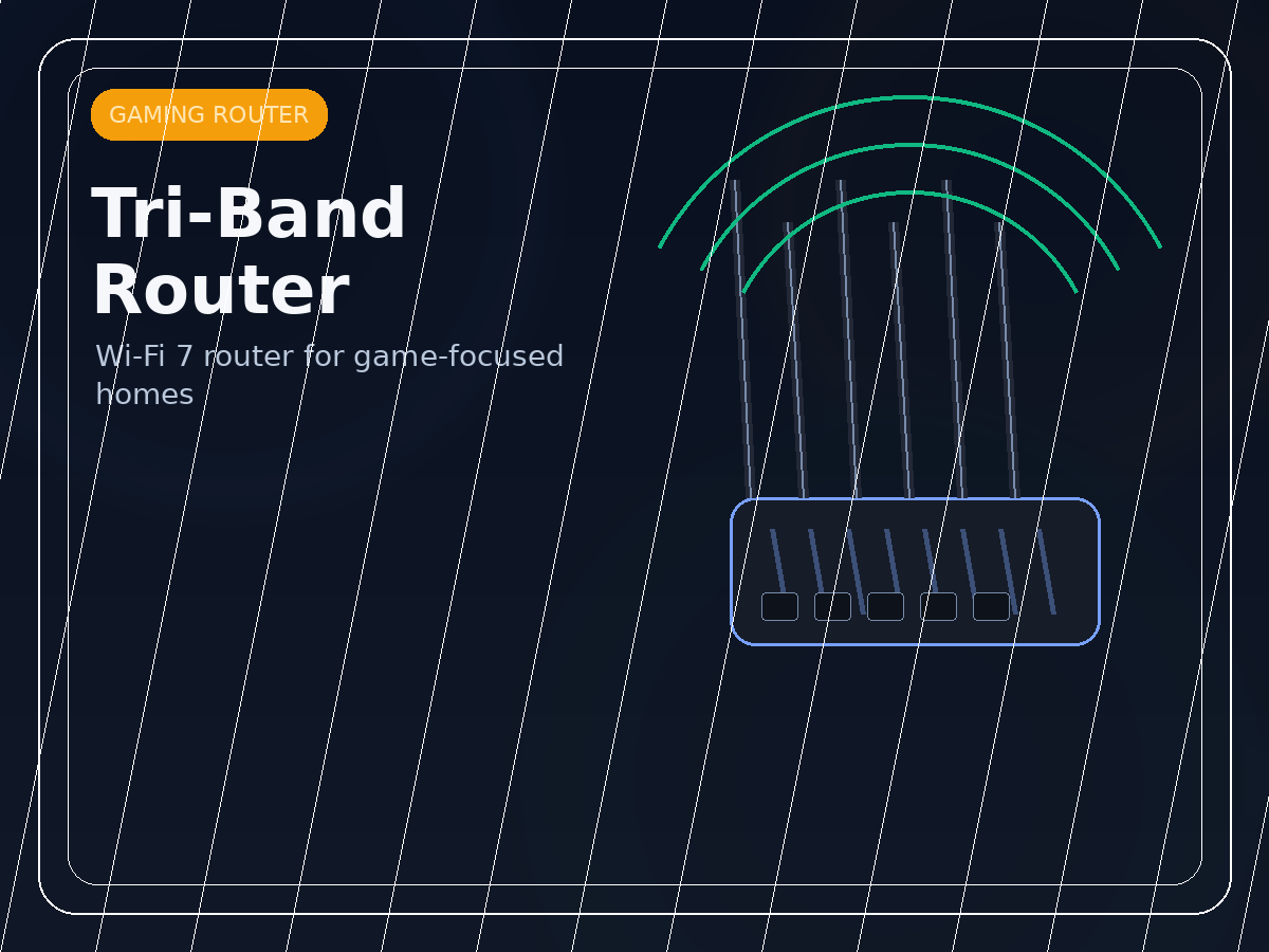
A gaming-router recommendation that fits comparison posts aimed at buyers who want WiFi 7, multi-gig ports, and dedicated gaming features at a lower price than flagship models.
- Tri-band BE11000 WiFi 7
- 320MHz support
- 2 x 5G plus 3 x 2.5G ports
- Dedicated gaming tools
- RGB gaming design
Why it stands out
- More approachable price tier
- Strong gaming-focused networking pitch
- Useful comparison option next to premium routers
Things to know
- Not as extreme as flagship router options
- Software preferences vary by buyer
Why connections sit at the center of geometry
On $\mathbb R^n$, a vector field is just a map $X:\mathbb R^n\to\mathbb R^n$, and you can differentiate it using ordinary partial derivatives. On a manifold, vectors live in different tangent spaces $T_pM$, so subtraction like $X(p)-X(q)$ is meaningless.
A connection repairs that by providing a covariant derivative
that tells you how the vector field $Y$ changes in the direction $X$, producing another vector field. The key feature is that $\nabla$ is local, linear in the direction field, and satisfies a Leibniz rule in the second slot.
With a connection in hand, you get:
- Geodesics: curves $\gamma$ with $\nabla_{\dot\gamma}\dot\gamma=0$.
- Parallel transport: vectors $V(t)$ along $\gamma$ with $\nabla_{\dot\gamma}V=0$.
- Curvature: the obstruction to second covariant derivatives commuting.
The mental model to keep is simple: a connection is a rule for comparing nearby tangent spaces, and curvature measures the failure of that comparison to be path-independent.
The Levi–Civita connection: the default choice
If $(M,g)$ is Riemannian, there is a unique connection $\nabla$ characterized by:
- Metric compatibility: $X\langle Y,Z\rangle = \langle \nabla_X Y, Z\rangle + \langle Y, \nabla_X Z\rangle$.
- Zero torsion: $\nabla_X Y – \nabla_Y X = [X,Y]$.
This is the Levi–Civita connection. Its existence and uniqueness are not just a theorem to cite; they are a proof tactic. Whenever a problem statement mentions only $g$, you should expect the Levi–Civita connection to be the intended mechanism.
A computational entry point is the Koszul formula:
You rarely compute with this directly on long problems, but it tells you what is allowed: anything about $\nabla$ must be built from $g$ and brackets of vector fields.
The proof strategy spine: translate, simplify, then use tensoriality
A reliable strategy for many geometry proofs looks like this:
- Translate the claim into an identity involving $\nabla$, curvature $R$, or parallel transport.
- Choose coordinates or frames where the connection simplifies at the point or along a curve.
- Use tensoriality to evaluate at a point in the simplest possible configuration.
- Only then compute.
The step that many people miss is tensoriality. Curvature, torsion, and many connection-derived objects are tensors in suitable slots, so you can compute them using any convenient extension of vectors to fields and any convenient coordinates at a point.
A small table of what you can normalize away
| Object | What you can arrange locally | What you cannot erase |
|—|—|—|
| Metric $g$ | $g_{ij}(p)=\delta_{ij}$ | curvature data |
| Connection $\nabla$ | $\Gamma^k_{ij}(p)=0$ in normal coordinates | derivatives of $\Gamma$ tied to curvature |
| Frame | orthonormal at $p$ | global twisting and topology |
| Curve $\gamma$ | arclength parametrization | curvature constraints on its image |
The habit to cultivate: normalize at the place where the main estimate or identity will be evaluated.
Curvature as a commutator identity
Curvature is defined by
This definition already suggests a proof move: if you can rewrite your statement as the vanishing of such a commutator, you are proving flatness or controlling curvature. If you can show the commutator has a definite sign in a quadratic form, you are proving comparison theorems or rigidity.
Even without full computations, the formal properties matter:
- $R(X,Y)$ is linear in each input and alternating in $X,Y$.
- For Levi–Civita connections, $R$ satisfies strong symmetry identities.
- Curvature controls the second variation of energy and hence geodesic stability.
You do not need to write down all symmetries to use them. Often it is enough to know that “curvature is a tensor,” so you can compute it in a well-chosen frame.
Worked example: great circles are geodesics on the sphere
Let $S^2\subset\mathbb R^3$ have the metric induced from the Euclidean inner product. A clean strategy avoids messy coordinates.
Take a smooth curve $\gamma(t)\in S^2$. View it as a curve in $\mathbb R^3$. The ambient derivative $\ddot\gamma$ decomposes into tangential and normal parts relative \to $S^2$.
The Levi–Civita connection on $S^2$ can be described as “differentiate in $\mathbb R^3$ and project to the tangent space.” Concretely,
the tangential component of $\ddot\gamma$.
So $\gamma$ is a geodesic exactly when $\ddot\gamma$ is normal to the sphere, meaning it is proportional \to $\gamma$ itself (because the normal direction at $\gamma$ is spanned by $\gamma$):
Now specialize \to a great circle. A great circle is the intersection of $S^2$ with a two-dimensional linear subspace $P\subset\mathbb R^3$ through the origin. Parametrize it by arclength so that $\gamma(t)\in P$ and $\|\gamma(t)\|=1$.
Within the plane $P$, $\gamma$ is a unit-speed circle, so $\ddot\gamma$ points toward the center, which is the origin. That means $\ddot\gamma$ is proportional \to $\gamma$ with negative coefficient. Therefore the tangential component is zero, so the curve is a geodesic.
This proof showcases a general pattern:
- Use a geometric description of the connection (projection from an ambient space).
- Convert “geodesic” \to “acceleration has no tangential component.”
- Reduce the claim to an elementary computation in a simpler space.
No heavy coordinate machinery is required, and the argument generalizes to many submanifold settings.
Strategy patterns you can reuse across geometry problems
These are not slogans. They are moves that tend to convert a complicated question into a short computation.
- Move: choose normal coordinates at a point.
If a statement is pointwise, set $\Gamma^k_{ij}(p)=0$ and evaluate there. What remains is curvature or tensor algebra, not connection clutter.
- Move: prove an identity for all vectors by checking it on a basis.
For bilinear expressions, choose an orthonormal basis at a point and compute components. This avoids global coordinate entanglement.
- Move: use parallel transport to compare tangent spaces.
If you need to compare vectors at different points, transport them along a curve and differentiate the transported quantity. This often reveals conserved quantities.
- Move: rewrite in terms of energy or length.
Many geometric claims about geodesics become calculus of variations statements. The connection provides the Euler–Lagrange equation $\nabla_{\dot\gamma}\dot\gamma=0$.
- Move: separate what is tensorial from what is coordinate-dependent.
Curvature is tensorial; Christoffel symbols are not. If your proof depends on Christoffel symbols in a way that is not obviously invariant, you are probably proving a coordinate artifact.
Reading geometry papers without drowning in notation
Geometry papers often compress a huge amount of structure into short expressions. A practical decoding approach is:
- Identify the connection being used: Levi–Civita, a principal bundle connection, or a chosen affine connection.
- Find the curvature object and its convention: $R(X,Y)Z$ can differ by sign between authors.
- Locate where tensoriality is exploited: many “miraculous simplifications” are just evaluations in normal coordinates.
- Track which statements are global and which are local; proofs often silently switch perspectives using coverings or compactness.
If you can keep those anchors, the rest is computation and bookkeeping, not mystery.
The moving-frames viewpoint: connections without coordinates
Coordinates are useful, but many of the cleanest geometric proofs avoid them entirely by using frames and differential forms. The connection becomes a matrix of one-forms, and curvature becomes a matrix of two-forms.
Choose an orthonormal frame $e_1,\dots,e_n$ on an open set. Define connection one-forms $\omega_{ij}$ by
Metric compatibility forces $\omega_{ij}=-\omega_{ji}$, so the connection lives in the Lie algebra of the orthogonal group.
Let $\theta^i$ be the dual coframe. Then the structure equations are:
- First structure equation (torsion-free condition in the Levi–Civita case):
- Second structure equation (curvature):
where $\Omega_{ij}$ are the curvature two-forms representing $R$ in the frame.
Why does this help with proofs? Because many statements are naturally about how things rotate as you move. Frames make rotation visible, and wedge products make antisymmetry automatic. If a coordinate calculation would involve pages of Christoffel symbols, the moving-frames version often collapses \to a line or two of exterior algebra plus one clever normalization.
A practical rule:
- Use coordinates when you need explicit components for an estimate.
- Use frames when you need structural identities and cancellations.
A global payoff: curvature integrates to topology
Once you are fluent with the connection language, you start recognizing that curvature does not only sit pointwise. It accumulates. The clearest instance on surfaces is the Gauss–Bonnet theorem, which relates the integral of Gaussian curvature to the Euler characteristic. You do not need the full formal statement here; what matters for proof strategy is the message:
- Connection and curvature let you convert local differential data into global invariants.
That is why “start with connections” is not merely advice about technique. It is advice about the bridge between local computations and global conclusions.
What starting with connections gives you
Connections are not only a technique; they are a proof architecture:
- They tell you what it means to differentiate geometric data.
- They unify geodesics, curvature, and transport into one language.
- They provide canonical normalizations that remove noise.
- They expose invariants that survive coordinate changes.
When geometry problems feel slippery, it is often because the tangent spaces are moving under your feet. A connection is the formal way to stop that movement long enough to calculate.
Books by Drew Higgins


Leave a Reply