Singular value decomposition (SVD) is the piece of linear algebra that most cleanly turns abstract statements into geometry you can draw and computations you can trust. It tells you what a matrix does to the unit sphere, how far it stretches in each principal direction, and which directions are crushed nearly to zero. That single perspective connects least squares, pseudoinverses, conditioning, low‑rank approximation, and a large portion of practical numerical linear algebra.
This article builds the SVD from the ground up, explains why it is the correct notion of diagonalization for rectangular or nonnormal matrices, and shows how to use it to reason about stability, error, and structure without hiding behind slogans.
Value WiFi 7 RouterTri-Band Gaming RouterTP-Link Tri-Band BE11000 Wi-Fi 7 Gaming Router Archer GE650
TP-Link Tri-Band BE11000 Wi-Fi 7 Gaming Router Archer GE650
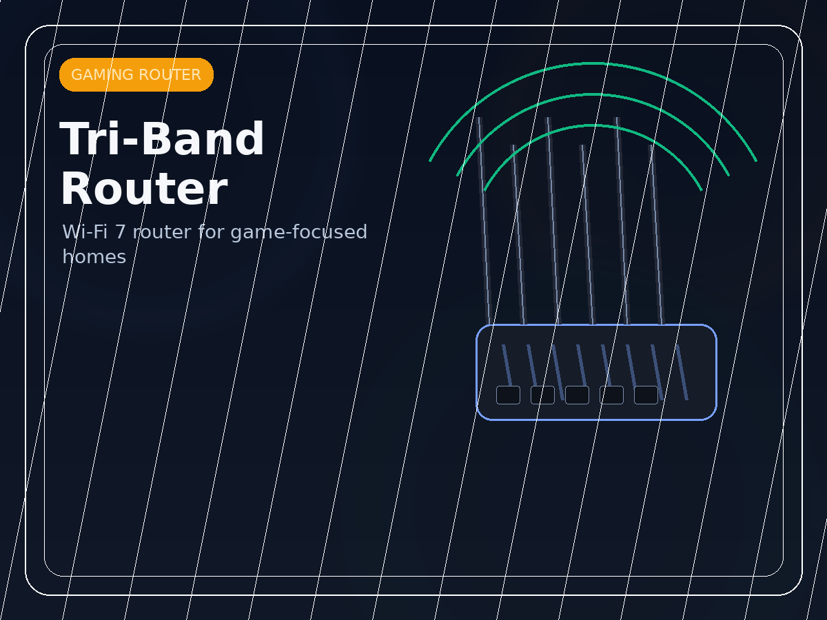
A gaming-router recommendation that fits comparison posts aimed at buyers who want WiFi 7, multi-gig ports, and dedicated gaming features at a lower price than flagship models.
- Tri-band BE11000 WiFi 7
- 320MHz support
- 2 x 5G plus 3 x 2.5G ports
- Dedicated gaming tools
- RGB gaming design
Why it stands out
- More approachable price tier
- Strong gaming-focused networking pitch
- Useful comparison option next to premium routers
Things to know
- Not as extreme as flagship router options
- Software preferences vary by buyer
What the SVD states and why it is the right normal form
Let $A$ be a real $m\times n$ matrix. The SVD says there exist orthogonal matrices $U\in\mathbb{R}^{m\times m}$ and $V\in\mathbb{R}^{n\times n}$, and a diagonal matrix
with $\sigma_1\ge\sigma_2\ge\cdots\ge\sigma_r>0$ and $r=\operatorname{rank}(A)$, such that
The diagonal entries $\sigma_i$ are the singular values. The columns $u_i$ of $U$ are left singular vectors, and the columns $v_i$ of $V$ are right singular vectors.
Two features make this decomposition the correct normal form for general matrices.
- It is always available, for every real matrix, square or rectangular.
- It is orthogonally invariant: multiplying $A$ on the left or right by an orthogonal matrix does not change its singular values, only rotates singular vectors.
That invariance aligns with geometry. Orthogonal transformations preserve lengths and angles. So the singular values are the intrinsic stretch factors of the linear map, independent of the coordinate system.
The unit sphere picture: ellipsoids and principal stretches
Consider the unit sphere $S^{n-1} = \{x\in\mathbb{R}^n : \|x\|_2=1\}$. The image of this sphere under $A$ is an ellipsoid in $\mathbb{R}^m$ (possibly flattened). The SVD identifies its principal axes.
From $A v_i = \sigma_i u_i$, we see that:
- each right singular vector $v_i$ is a direction in the domain,
- $A$ sends $v_i$ \to a vector in the codomain aligned with $u_i$,
- the length of that image is exactly $\sigma_i$.
So the ellipsoid has semiaxis lengths $\sigma_1,\dots,\sigma_r$ along directions $u_1,\dots,u_r$, and any component of the input in the nullspace direction is mapped to zero.
A helpful consequence is an exact variational characterization:
More generally, the set of singular values controls every induced Euclidean operator norm you care about.
How to derive the SVD from symmetric matrices
The SVD is often presented as a fact to memorize, but it is better understood as a consequence of spectral theory for symmetric matrices.
Start with $A^{\mathsf T}A$, which is an $n\times n$ symmetric positive semidefinite matrix. Therefore it has an orthonormal eigenbasis:
Define $\sigma_i = \sqrt{\lambda_i}$. For each eigenvector with $\sigma_i>0$, define
Then $u_i$ has unit length because
One can also check orthogonality: distinct eigenvectors of $A^{\mathsf T}A$ are orthogonal, and the corresponding $u_i$ become orthogonal as well. Completing $\{u_i\}$ \to an orthonormal basis of $\mathbb{R}^m$ yields $U$, and taking $V$ as the eigenvector matrix yields the decomposition.
This proof matters because it reveals a chain of ideas.
- SVD reduces to diagonalizing a symmetric matrix.
- Singular values are square roots of eigenvalues of $A^{\mathsf T}A$ and $A A^{\mathsf T}$.
- Numerical methods for symmetric eigenproblems become methods for SVD.
Rank, nullspace, and the four fundamental subspaces
SVD organizes the classical four subspaces picture in a way that is computationally concrete.
Let $A = U\Sigma V^{\mathsf T}$ and $r=\operatorname{rank}(A)$.
- The column space $\operatorname{Col}(A)$ is spanned by the first $r$ columns of $U$.
- The row space $\operatorname{Row}(A)$ is spanned by the first $r$ columns of $V$.
- The nullspace $\mathcal{N}(A)$ is spanned by the last $n-r$ columns of $V$.
- The left nullspace $\mathcal{N}(A^{\mathsf T})$ is spanned by the last $m-r$ columns of $U$.
This is not only conceptual; it is actionable. If you want a stable basis for the nullspace, the last right singular vectors provide one. If you want an orthonormal basis for the range, the first left singular vectors provide one.
The SVD also makes orthogonal projectors explicit:
where $U_r$ and $V_r$ collect the first $r$ singular vectors.
Least squares, pseudoinverses, and what the solution really is
Least squares problems appear everywhere: fit a model, solve an inconsistent linear system, recover a signal. Given $A\in\mathbb{R}^{m\times n}$ and $b\in\mathbb{R}^m$, the least squares problem is
If $A$ has full column rank, the normal equations $A^{\mathsf T}A x = A^{\mathsf T}b$ have a unique solution. But using the normal equations directly squares the condition number and can be numerically fragile. The SVD provides a clearer and safer representation.
Write $A = U\Sigma V^{\mathsf T}$. Then
because $U$ is orthogonal. Let $y = V^{\mathsf T}x$ and $c = U^{\mathsf T}b$. The problem becomes
Since $\Sigma$ is diagonal, the minimization decouples coordinatewise. For $i\le r$, the best choice is $y_i = c_i/\sigma_i$. For $i>r$, the choice of $y_i$ does not affect the residual because those directions lie in the nullspace. The minimum‑norm solution sets them to zero.
This yields the Moore–Penrose pseudoinverse:
where $\Sigma^+$ has diagonal entries $1/\sigma_i$ for $i\le r$ and zeros elsewhere. The minimum‑norm least squares solution is $x_* = A^+ b$.
A table captures what the pseudoinverse does in each singular direction.
| Direction in domain | Matrix action | Contribution to solution |
|—|—|—|
| $v_i$ with large $\sigma_i$ | strong, stable stretch | $y_i=c_i/\sigma_i$ stays controlled |
| $v_i$ with tiny $\sigma_i$ | near‑collapse | $y_i=c_i/\sigma_i$ can blow up, amplifying noise |
| nullspace directions | mapped to zero | set to zero for minimum norm |
This table is the moral reason SVD is central to inverse problems: small singular values are where instability lives.
Conditioning: the honest measure of sensitivity
For a square invertible matrix $A$, the 2‑norm condition number is
A large condition number means small perturbations in $b$ or rounding in computation can cause large changes in the solution of $Ax=b$.
The SVD explains this without handwaving. In the coordinates $y = V^{\mathsf T}x$, solving $Ax=b$ becomes $\Sigma y = U^{\mathsf T}b$. Each coordinate divides by $\sigma_i$. If $\sigma_n$ is tiny, division amplifies errors in that coordinate.
One practical response is regularization. A common choice is Tikhonov (ridge) regularization:
In SVD coordinates, this becomes
Small singular directions are damped instead of amplified. The parameter $\lambda$ trades bias for stability.
Best low‑rank approximation and the meaning of “signal”
Suppose you want to approximate $A$ by a matrix of rank at most $k$, perhaps for compression or noise reduction. The SVD gives the best answer in the 2‑norm and Frobenius norm.
Write
The truncated SVD
is the best rank‑$k$ approximation, with errors
This theorem (Eckart–Young–Mirsky) says singular values measure the energy of the matrix across orthogonal modes. Keeping the largest $k$ modes preserves as much as possible, while discarding the smallest modes removes directions that contribute least in a normed sense.
A practical interpretation stays close to geometry.
- If $\sigma_{k+1}$ is much smaller than $\sigma_k$, the matrix has an effective rank near $k$.
- If the singular values decay slowly, compression requires losing significant structure.
Polar decomposition: separating rotation and stretch
Another perspective that clarifies geometry is polar decomposition. For any $A\in\mathbb{R}^{m\times n}$, one can write
where $Q$ has orthonormal columns (a partial isometry) and $H = (A^{\mathsf T}A)^{1/2}$ is symmetric positive semidefinite.
Using the SVD, the stretch part is $H = V\Sigma^{\mathsf T}\Sigma V^{\mathsf T}$ square‑rooted, and the length‑preserving part is built from the singular vector frames. Conceptually:
- $H$ is the pure stretch in the domain directions.
- $Q$ is the length‑preserving transformation that places that stretched object into the codomain.
This separation prevents common conceptual mistakes. Many complicated matrices are not mysterious rotations with some scaling added. They are rotations composed with a symmetric stretch.
A worked micro‑example you can compute by hand
Take
Compute
The eigenvalues of this symmetric matrix are
So the singular values are
The corresponding eigenvectors (normalized) give $V$. Then $u_i = Av_i/\sigma_i$ gives the left singular vectors. Even in this small example, the point is visible: the singular values are not arbitrary constants; they are forced by the symmetric form $A^{\mathsf T}A$, and they quantify the stretching of the unit circle into an ellipse.
Practical takeaways that stay true across contexts
SVD is not merely a decomposition, it is a method for asking stable questions.
- If you need a reliable basis for a subspace attached \to $A$, use singular vectors.
- If you care about sensitivity, look at the ratio $\sigma_1/\sigma_r$ over the active rank.
- If a computed solution is unstable, inspect small singular values rather than guessing.
- If you need to compress or denoise a matrix, truncate the SVD and measure the discarded tail.
Linear algebra is often taught as manipulation of symbols. SVD returns it to its true content: geometry of linear maps with a numerical conscience. Once you internalize that the singular values are the axes of the image ellipsoid, many puzzles of least squares and instability stop being puzzles and become visible.
Books by Drew Higgins


Prophecy and Its Meaning for Today
New Testament Prophecies and Their Meaning for Today
A focused study of New Testament prophecy and why it still matters for believers now.

Leave a Reply